Antenna Gain Formula and dBi Guide

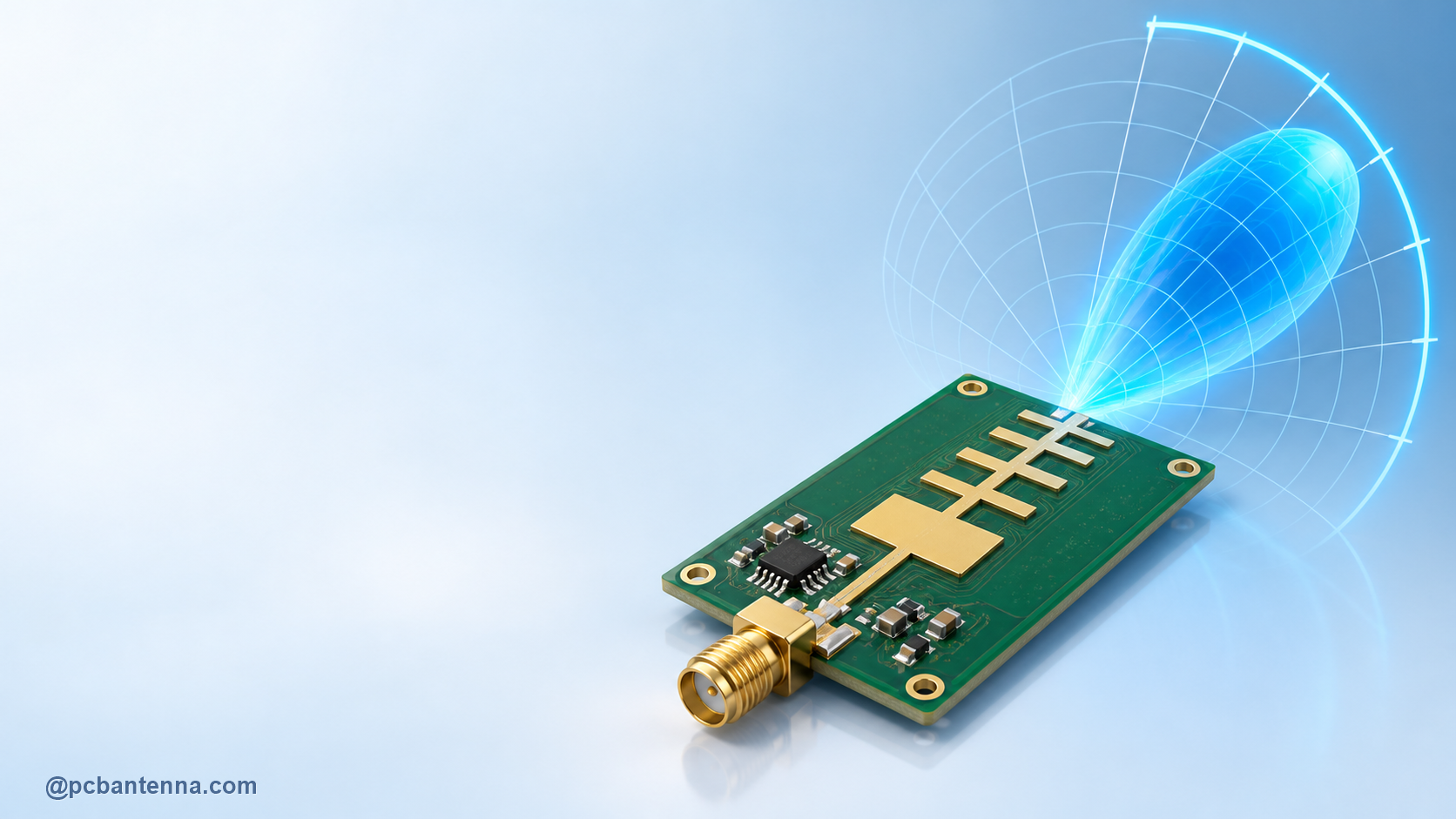
Antenna gain is one of the first numbers people compare, and one of the easiest to misread. A larger dBi value does not create power. It describes how effectively an antenna concentrates radiation in a particular direction compared with an ideal isotropic reference. That concentration can help a link in one direction, while making coverage worse somewhere else.

The antenna gain formula becomes much more useful when you connect it to directivity, efficiency, effective aperture, and a real link budget. This guide keeps the math practical, explains the difference between linear gain and dBi, and shows how to use the result without overpromising range.

The core antenna gain formula

In linear units, antenna gain is commonly expressed as:

G = η × D

Here, G is gain, D is directivity, and η is radiation efficiency as a linear number between 0 and 1. Directivity tells you how strongly the antenna focuses its radiation in a chosen direction compared with radiation averaged over all directions. Efficiency accounts for power that is lost as heat or otherwise does not become radiated energy. Ansys and Keysight both describe gain as directivity scaled by antenna efficiency.

For example, an antenna with a linear directivity of 4 and radiation efficiency of 0.70 has linear gain of 2.8. The formula is simple, but do the multiplication in linear units first. Decibels are logarithmic, so multiplying linear values becomes addition only after converting each term to dB.

From linear gain to dBi

Datasheets usually show gain in dBi, meaning decibels relative to an ideal isotropic radiator. Convert a linear gain value with:

G(dBi) = 10 log10(G linear)

Using the example above, 10 log10(2.8) is about 4.5 dBi. The inverse calculation is:

G linear = 10^(G(dBi) / 10)

A value below 0 dBi is not automatically bad. It means the antenna’s peak response is lower than the isotropic reference after the relevant losses are included. Small embedded antennas often make deliberate compromises among physical size, bandwidth, efficiency, pattern shape, enclosure effects, and cost. The useful comparison is against the product requirement, not against a generic “higher is better” target.

Directivity, gain, and realized gain are not interchangeable

These terms are closely related, but they answer different questions:

• Directivity describes how concentrated the radiation pattern is, without conductor and dielectric loss.
• Gain includes radiation efficiency, so it is lower than directivity when the antenna has loss.
• Realized gain also includes input mismatch, making it especially useful when the antenna is evaluated with its actual feed and match.

HFSS can report peak directivity, gain, and peak realized gain as separate antenna parameters. A large gap between directivity and realized gain is a cue to look at both loss and mismatch. Start with the HFSS S11 simulation setup, then inspect the far-field response with our HFSS far-field pattern guide.

Efficiency in dB and percent

Efficiency is often reported as a percentage or a decimal. An efficiency of 70% is 0.70 in the gain formula. To express an efficiency factor in dB, use 10 log10(η). For 70%, that is about -1.55 dB. If the directivity is 6 dBi, the corresponding gain before mismatch would be about 4.45 dBi.

That negative efficiency term is normal. It is a loss term, not an extra signal source. Copper loss, dielectric loss, nearby lossy materials, and an electrically small radiator can all contribute. In a compact PCB design, the ground plane and product mechanics often affect both efficiency and pattern. Use the PCB antenna ground-plane guide before judging an antenna trace in isolation.

The effective aperture formula

Gain also connects an antenna’s transmit and receive behavior through effective aperture. The common relation is:

Ae = (λ² × G) / (4π)

Ae is effective aperture in square metres, λ is wavelength in metres, and G is linear gain. Rearranged, it becomes G = 4πAe / λ². This does not mean a physically small antenna secretly has a large physical capture area. Effective aperture is a receive-performance concept that depends on frequency, direction, polarization match, and antenna behavior.

The wavelength term explains why frequency matters. A gain value without its frequency is incomplete. The same geometry can produce a very different result when the operating band changes. You can use the RF and antenna calculators to quickly check wavelength before working through a receiving-area or link-budget estimate.

How gain appears in a link budget

A basic free-space link budget usually adds transmit power and antenna gains, then subtracts path loss and other losses:

Pr(dBm) = Pt(dBm) + Gt(dBi) + Gr(dBi) – path loss(dB) – other losses(dB)

“Other losses” can include cable loss, connector loss, polarization mismatch, fading margin, and implementation loss. The equation is useful bookkeeping, but it is not a promise of field range. A real indoor link sees multipath, orientation changes, human proximity, walls, and receiver sensitivity limits. A high-gain antenna can help a fixed point-to-point path while producing a coverage hole for a mobile product.

Imagine two 2.4 GHz antennas in a controlled test. Replacing a 1 dBi transmit antenna with a 4 dBi antenna changes only one term in the idealized link budget: it adds roughly 3 dB in the direction where that gain is specified. Whether the receiver sees that improvement depends on alignment, polarization, the rest of the pattern, and the environment. Check the radiation pattern before translating a peak-gain number into a coverage claim.

dBi versus dBd

dBi uses an isotropic radiator as the reference. dBd uses a half-wave dipole as the reference. In free space, a half-wave dipole has about 2.15 dB more gain than an isotropic radiator, so the usual conversion is:

Gain(dBi) = Gain(dBd) + 2.15 dB

Always confirm the reference before comparing numbers from two suppliers. A 3 dBd antenna and a 3 dBi antenna do not describe the same peak gain. Our companion antenna gain guide covers this comparison with more context.

A practical workflow for PCB antennas

1. Define the frequency band, orientations, and coverage requirement before setting a gain target.
2. Simulate S11, radiation efficiency, realized gain, and the full pattern in the intended board and enclosure configuration.
3. Compare the same frequency, polarization, and angular cut across revisions.
4. Use peak gain together with null depth and coverage direction, not as a stand-alone score.
5. Measure representative hardware and investigate meaningful gaps between simulated and measured results.
6. Add link margin for the actual product environment instead of assuming ideal free-space behavior.

Common gain calculation mistakes

• Adding or multiplying dB values using linear-unit rules.
• Using percent efficiency directly instead of converting 70% to 0.70.
• Comparing dBd and dBi without converting the reference.
• Using directivity as if it already includes material loss and mismatch.
• Quoting a peak value without the frequency, plane, polarization, and pattern context.
• Assuming a 3 dB peak-gain increase will improve every product orientation by 3 dB.

The takeaway

The antenna gain formula is compact: gain equals directivity times efficiency. Its engineering value comes from the surrounding questions: which direction, which frequency, what efficiency definition, how much mismatch, and what happens inside the finished product? Use linear values for the physics, dB values for a link budget, and real pattern data for the coverage decision. When a PCB antenna needs more than a quick estimate, contact PCB Antenna for simulation, layout, and validation support.

References and further reading

• Keysight: Introduction to Antenna Theory and Antenna Measurement Fundamentals.
• Ansys: Radio-frequency simulation methodology.
• Antenna-Theory.com: Effective Aperture.